
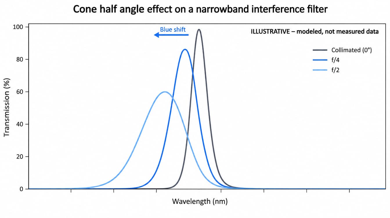
- A cone half angle shifts an interference filter’s spectrum toward shorter wavelengths and softens its edges; a pure tilt only shifts it.
- With the chief ray normal and a uniformly filled pupil, the mean shift equals half the marginal-ray shift.
- The same cone produces far more spectral spread when it is centered on a tilted chief ray.
- Verify by averaging collimated angle-resolved data in linear transmittance, then confirm on a bench at the working f-number.
- Specify cone half angle, chief-ray angle range and the acceptance route as separate items.
A cone half angle makes an interference filter see a spread of incidence angles at once. The spectrum shifts toward shorter wavelengths, edges soften, and peak transmission drops once the angular spread approaches the passband width. You verify the cone half angle effect on interference filters by averaging collimated angle-resolved data over the real ray distribution, then confirming it at the system’s working f-number.
Cone half angle (CHA) is the angle between the axis of a converging or diverging beam and its outermost ray at the filter. A CHA of 0° means collimated light. The effect matters most for narrowband filters and steep edge filters placed in non-collimated space: near a focal plane, after a fiber, or directly in front of a sensor. The underlying mechanism is the same one behind the angle-of-incidence behavior of thin-film filters. The difference is that a cone mixes many angles into one measured curve.
What does a cone half angle do to an interference filter spectrum?
Every ray in the cone crosses the coating at its own angle, and each angle shifts the spectrum toward shorter wavelengths by a different amount. The response seen by the detector is the average of all those shifted spectra, weighted by how much light each angle carries. The net result is a blue shift smaller than a tilt to the marginal-ray angle would produce, together with a broadening that a tilt alone does not cause.
In a measured or calculated curve, the cone shows up as five linked changes:
- The center wavelength (CWL) and edge positions move to shorter wavelengths.
- The passband widens and edge slopes decrease, because each edge becomes a blend of edges at different positions.
- Peak transmission falls once the spread of shifts becomes comparable to the FWHM.
- Passband ripple is smoothed out.
- Blocking just outside the band degrades, because rays shifted by larger angles leak light into wavelengths that the collimated design blocks.
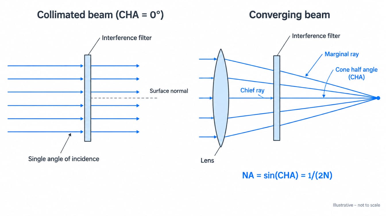
How are f-number, NA and cone half angle related?
For a beam in air, numerical aperture equals the sine of the cone half angle. For an aplanatic system focusing at infinite conjugate, NA = 1/(2N), where N is the working f-number. An f/2 beam therefore has NA 0.25 and a cone half angle of 14.5°.
The paraxial form tan(CHA) = 1/(2N) gives 14.0° for the same f/2 beam. The difference grows with faster beams, so a specification should state which relation was used. At finite conjugates, use the working f-number. With unit pupil magnification, the working f-number is N(1 + |m|), which is larger than the infinity-focus value.
Numerical aperture is conserved across planar interfaces: n0·sin θ0 stays constant as light passes from air into a cemented or immersed filter. The spectral shift depends on this product, not on the geometric angle inside a particular medium. For that reason, NA is the clearest way to hand a cone condition from an optical designer to a coating designer.
How large is the cone-induced shift?
The shift for a single ray follows λ(θ) = λ0·√(1 − (n0·sin θ0 / neff)²), where λ0 is the wavelength of a spectral feature at normal incidence and neff is the effective index of the coating for that feature. For a cone, the size of the shift is set by the NA, the wavelength and neff, while its distribution is set by how the pupil is illuminated.
neff is not the refractive index of any single coating material. It depends on the layer design. In a cavity bandpass filter, for example, the spacer material has a strong influence on it, and it can differ between the passband and the edges of the same filter. A higher neff means a smaller shift for the same angle.
For small angles, the shift of a ray is proportional to the square of its NA: Δλ ≈ λ0·NA²/(2·neff²). Suppose the chief ray is normal to the filter and the circular pupil is uniformly filled. The light carried by each annulus of the pupil grows in proportion to its radius, and the shift grows with the square of that radius. These two factors cancel, so the shifts are spread uniformly between zero and the marginal-ray value. Two consequences follow:
- The mean shift equals half the shift of the marginal ray.
- The filter behaves as if its collimated curve were shifted by that mean and then convolved with a rectangular kernel whose width equals the marginal-ray shift.
| Working f/# | NA | CHA | Max shift (1.8) | Mean shift (1.8) | Max shift (2.1) |
|---|---|---|---|---|---|
| f/8 | 0.063 | 3.6° | 0.51 nm | 0.26 nm | 0.38 nm |
| f/4 | 0.125 | 7.2° | 2.05 nm | 1.03 nm | 1.51 nm |
| f/2.8 | 0.179 | 10.3° | 4.19 nm | 2.09 nm | 3.08 nm |
| f/2 | 0.250 | 14.5° | 8.24 nm | 4.11 nm | 6.04 nm |
| f/1.4 | 0.357 | 20.9° | 16.90 nm | 8.42 nm | 12.38 nm |
The table values are calculated, not measured product data. Calculation conditions: λ0 = 850 nm; neff = 1.8 or 2.1, used as illustrative assumptions; incidence from air; chief ray normal to the filter; uniformly filled circular pupil; NA = 1/(2N); polarization-averaged; rigid-shift model with neff held constant over the angle range. “Max shift” is the marginal-ray shift. “Mean shift” is the pupil-weighted average.
How much peak transmission is lost depends on the shape of the passband. For a single-cavity filter with a Lorentzian-like passband of FWHM w, averaging over a uniform shift spread of width D centered on the peak leaves a peak of (w/D)·arctan(D/w) relative to the collimated peak. That works out to 0.93 at D = 0.5w, 0.79 at D = w, and 0.55 at D = 2w. A multi-cavity filter with a flat top holds its peak until D approaches the width of the flat region, but each edge still widens by D.
Why does a cone on a tilted filter broaden more than a cone at normal incidence?
Because the shift grows with the square of the angle, a given angular spread produces a larger wavelength spread when it is centered on a tilted chief ray. At normal incidence, a cone of NA α spreads shifts over λ0·α²/(2·neff²). With a chief ray at angle θc ≥ α, the spread becomes roughly 2·λ0·θc·α/neff² in the small-angle limit.
A calculated example shows the size of the difference. Take an 850 nm feature with neff = 1.8 and an f/4 cone. At normal incidence, the shifts span 0 to 2.1 nm. Center the same cone on a 10° chief ray and the shifts span 0.3 to 11.5 nm, a spread of 11.2 nm. The rays in the plane of tilt set these limits. Tilt also brings in s/p splitting. For a rotationally symmetric cone centered on the normal, s and p contributions average out over azimuth, even for linearly polarized input. Once the chief ray is tilted, that symmetry is lost.
This matters in non-telecentric image space. There, the chief ray angle changes with field position, so the filter passband changes across the image. A published Sandia analysis of infrared filters placed near a cooled focal plane treats exactly this case. It shows that the curve shape changes substantially, not just the center position.
| Illumination | Mean shift | Shift spread | Shape change | Polarization |
|---|---|---|---|---|
| Collimated, 0° AOI | None (reference) | None | None | No s/p splitting |
| Collimated, tilted | Set by AOI and neff | None within one polarization | From s/p splitting as AOI grows | s and p shift by different amounts |
| Cone, chief ray normal | Half the marginal-ray shift | 0 to marginal-ray shift | Softer edges, lower narrowband peak | Averaged by azimuthal symmetry |
| Cone, chief ray tilted | Close to the chief-ray shift | Grows with chief-ray angle × cone NA | Strongest broadening | s/p splitting present |
How do you verify the cone effect by calculation?
Calculation is the practical first check because it uses data that is normally available: a collimated spectrum and an effective index. Split the ray bundle into groups of nearly equal incidence angle. Rescale the wavelength axis for each group, weight each group by its share of the pupil, and sum the results. The output is the curve the system will actually see.
- Obtain the collimated normal-incidence spectrum, either measured or from the design file. Record the instrument’s beam geometry, polarization and spectral resolution with it.
- Obtain neff for the spectral feature that matters, either from the coating design or from a tilt measurement (see below). If the system has a tilted chief ray, use separate s and p values.
- Take the ray-angle distribution from the optical design: working f-number, chief-ray angle at each field point, pupil illumination profile, central obscuration and vignetting. For off-axis fields, a ray trace is more reliable than a formula.
- For each angle group i, multiply the wavelength axis by √(1 − (NAi/neff)²). Then multiply transmittance by the group’s weight and interpolate every group onto a common wavelength grid.
- Sum in linear transmittance, and convert to optical density only after summing. A small fraction of rays that leak strongly dominates the blocking result, so averaging OD values gives a result that is too optimistic.
- Compare the transformed curve with acceptance limits that were defined for the system condition, not for the collimated condition.
How to measure the effective index from tilt data
Measure the feature position at 0° and at several tilt angles in a well-collimated beam. For incidence from air, neff = sin θ / √(1 − (λθ/λ0)²) at each angle. Fitting several angles gives a more reliable value than a single pair of measurements. Measure s and p separately if they diverge over the angle range. Use angles that cover the system’s NA range, because neff derived at large tilts may not describe small angles well.
When the rigid-shift model is not enough
The rigid-shift model assumes that the curve keeps its shape at each angle and only moves. That assumption weakens as angles grow. Bandwidth, edge slope and s/p separation all change with angle, and neff itself can drift. For fast beams, strongly tilted chief rays or designs with steep edges, the coating designer should run a full angle-resolved thin-film calculation from the layer design and apply the pupil weighting to those results.
How do you verify it by direct measurement?
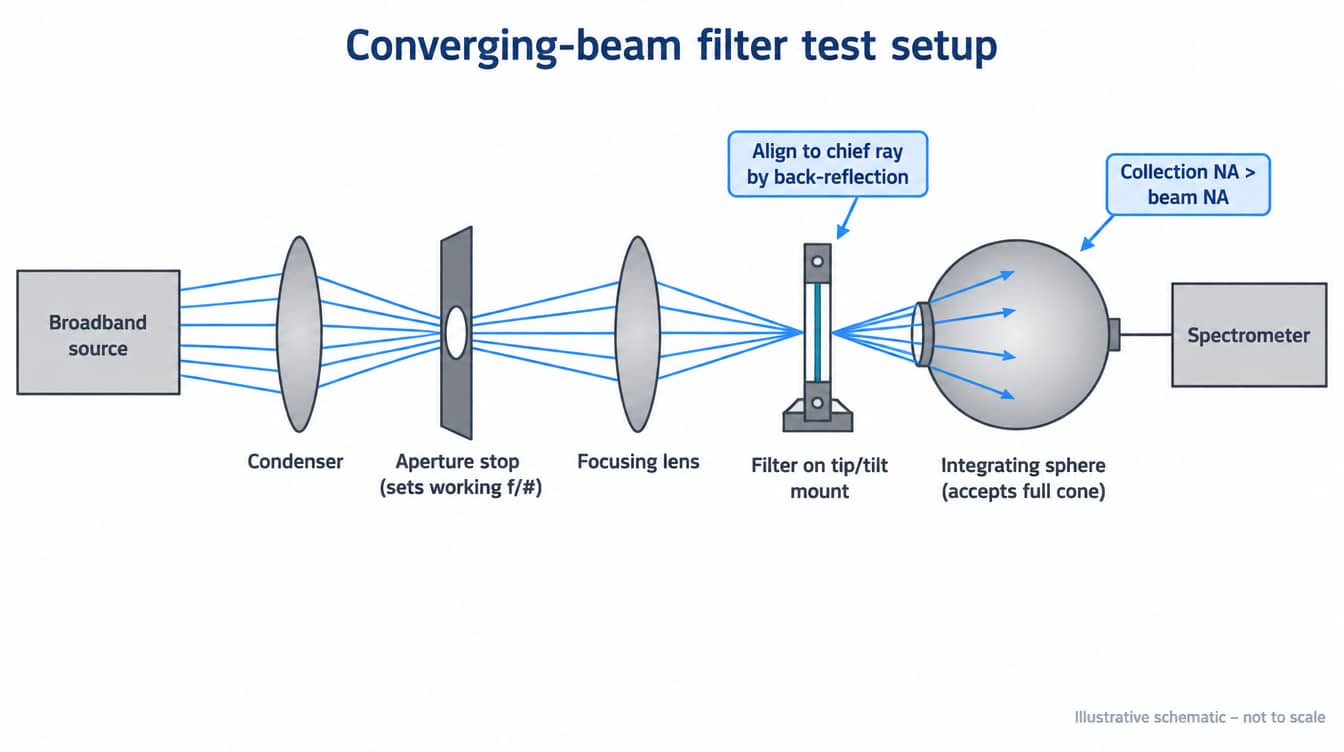
A direct test reproduces the system cone at the filter and records the spectrum with a detector that accepts all of it. Most commercial spectrophotometers do not offer an adjustable cone angle, and their sample beam has a fixed convergence of its own. Direct verification is therefore usually done on a bench setup built for the job.
- Beam definition: a broadband source and condenser, with an aperture stop that sets the working f-number. Confirm the actual NA by measuring the beam diameter at a known distance from focus.
- Filter mount: tip/tilt adjustment, aligned to the chief ray by back-reflection. A small residual tilt adds a chief-ray term that the calculation above shows is significant.
- Collection: an integrating sphere, or collection optics or fiber with an acceptance NA larger than the beam NA. A detector that clips the outer rays removes exactly the angles that cause the effect.
- Spectrometer: resolution finer than the features under test, so the instrument does not add its own broadening.
- Baseline: a reference scan without the filter, in the same geometry, to normalize the result.
A plane-parallel filter in a converging beam moves the focus downstream by t·(1 − 1/n) in the paraxial limit, where t is the filter thickness and n its substrate index. With fiber-coupled collection, refocus after inserting the filter. Otherwise the coupled NA changes and the result is biased. Record the pupil illumination profile too, because a Gaussian-weighted beam from a laser or a partly filled fiber carries less light at the marginal angles than a uniformly filled pupil.
Where the filter is already installed, an in-system check can replace the bench. Sweep a monochromator, or use narrow emission lines, at several field positions, and compare the measured system response with the calculated transform. Treat agreement between the two methods as the verification. Treat a disagreement as a sign that the ray-angle input, neff or the collection geometry needs rechecking. For how test conditions are tied to acceptance limits in a project, see our quality assurance approach.
What are the trade-offs when designing around a cone?
Each compensation corrects one symptom and moves the cost somewhere else. None of them removes broadening except avoiding the cone altogether.
- Pre-shift the design to a longer CWL. This puts the mean position on target at one f-number. The broadening remains. The collimated test curve then sits away from the system CWL, so acceptance has to reference the transformed curve. A variable iris or zoom breaks the compensation.
- Widen the FWHM. A wider band tolerates the shift spread with less peak loss. It also admits more background and weakens rejection close to the band.
- Use a design with higher neff. Angle sensitivity scales with 1/neff², so this reduces both mean shift and spread. What is achievable depends on the coating materials and on the other spectral targets of the design.
- Stop down the system. The cone NA scales with 1/N and the shift with 1/N². Image-plane irradiance also falls as 1/N², so signal is traded for spectral fidelity.
- Move the filter into collimated space. This removes the cone. In front of an imaging lens, however, each field point becomes a collimated beam at the field angle, so AOI now varies across the field. A filter placed there may also need a larger clear aperture.
- Use image-space telecentric optics. This holds the chief-ray angle near normal across the field, which removes the tilted-cone penalty. The cone itself remains.
Common mistakes when verifying cone angle performance
Most failures come from describing the cone incompletely or measuring it in a way that hides it. The following errors appear repeatedly in specifications and test reports.
- Writing the cone as an AOI range. “0–10°” says nothing about weighting, and it does not separate tilt from spread. State the chief-ray angle and the cone half angle (or NA) as two parameters.
- Accepting on the collimated curve alone. A filter that meets its CWL at 0° can miss the system target by the mean shift and fail its FWHM limit through broadening.
- Using the marginal-ray shift as the effective shift. For a normal chief ray and a uniform pupil, this overstates the mean shift by a factor of two. Using only the chief ray has the opposite problem: it ignores broadening entirely.
- Averaging optical density instead of transmittance. Blocking must be computed from averaged linear transmittance.
- Collecting less than the full cone. An undersized detector or fiber NA clips the high-angle rays and makes the filter look better than it will perform.
- Using the infinity f-number at finite conjugates. The working f-number sets the cone.
- Applying one neff to every feature. The passband, the edges and each polarization can each have a different value.
What should a cone half angle filter specification include?
A complete specification describes the light the filter will receive and states how conformance will be demonstrated. Without both, the supplier and the buyer can measure the same part and reach different conclusions. The list below applies to bandpass, edge and notch filters used in non-collimated space.
- Spectral targets (CWL, FWHM, edge positions, blocking), each with the condition it applies to: collimated at 0°, or at the system cone.
- Working f-number, NA or cone half angle, plus the relation used to convert between them.
- Chief-ray angle, or its range across the field.
- Incident medium, if the filter is cemented or immersed.
- Polarization state of the incident light.
- Pupil illumination profile, if it is not uniform.
- Acceptance route: a collimated measurement with an agreed transform, a direct cone measurement, or both.
- Reference measurement conditions: instrument beam geometry, polarization and spectral resolution.
Agreeing on these items at the requirement stage is part of any custom optics project review. Changing the acceptance route after parts are coated usually costs more than settling it before the design is finalized.
Frequently asked questions
What is cone half angle in an optical filter?
Cone half angle (CHA) is the angle between the axis of a converging or diverging beam and its outermost ray at the filter. A CHA of 0° means collimated light. For a beam in air, the sine of the cone half angle equals the numerical aperture, so an f/2 beam with NA 0.25 has a cone half angle of 14.5°.
How does cone half angle affect filter transmission?
A cone half angle makes an interference filter respond to many incidence angles at once. Each angle shifts the spectrum to shorter wavelengths by a different amount, so the combined curve moves blue, its edges become less steep and its passband widens. When the spread of shifts approaches the filter’s FWHM, peak transmission falls. Narrowband filters and steep edge filters show the effect first.
How do you convert f-number to cone half angle?
For a beam focused in air by an aplanatic system at infinite conjugate, numerical aperture equals 1/(2N), where N is the working f-number, and the cone half angle is arcsin(NA). An f/4 beam therefore has NA 0.125 and a cone half angle of 7.2°. At finite conjugates, use the working f-number, which is larger than the infinity-focus f-number.
Is cone half angle the same as angle of incidence?
Cone half angle and angle of incidence are separate parameters. Angle of incidence describes the tilt of a collimated beam, or of the chief ray, relative to the filter normal. Cone half angle describes the spread of ray angles around that chief ray. A tilt shifts the whole spectrum; a cone shifts it by a smaller average amount and also broadens it, so a filter specification should state both.
Can a spectrophotometer measure a filter at a specific cone angle?
Most commercial spectrophotometers do not offer an adjustable cone angle, and their sample beam has its own fixed convergence. Cone performance is therefore usually verified by calculation from collimated angle-resolved data, then confirmed on a bench setup that reproduces the system’s working f-number, with a detector or integrating sphere that collects the full cone.
How much does a converging beam shift a bandpass filter?
The shift depends on numerical aperture, center wavelength and the coating’s effective index. With the chief ray normal to the filter and a uniformly filled pupil, the mean shift is half the shift of the marginal ray. For an 850 nm filter with an assumed effective index of 1.8, an f/2 beam gives a calculated mean shift of 4.1 nm and a marginal-ray shift of 8.2 nm.
References
- H. A. Macleod, Thin-Film Optical Filters, CRC Press.
- P. H. Lissberger and W. L. Wilcock, “Properties of All-Dielectric Interference Filters. II. Filters in Parallel Beams of Light Incident Obliquely and in Convergent Beams,” Journal of the Optical Society of America 49, 126–130 (1959).
- C. R. Pidgeon and S. D. Smith, “Resolving Power of Multilayer Filters in Nonparallel Light,” Journal of the Optical Society of America 54, 1459–1466 (1964).
- Sandia National Laboratories, “Transformation of filter transmission data for f-number and chief ray angle,” U.S. DOE Office of Scientific and Technical Information, OSTI ID 671892, https://www.osti.gov/servlets/purl/671892
- ISO 15368, Optics and photonics — Measurement of reflectance of plane surfaces and transmittance of plane parallel elements.
If a filter will operate in a converging beam, send the drawing, optical specification or sample to GIAI for technical review. Include the wavelength range, substrate, dimensions, coating requirements, AOI together with the cone half angle or working f-number, inspection criteria and expected quantity.