
Technical Resources
F-Theta Scan Field Size Calculation
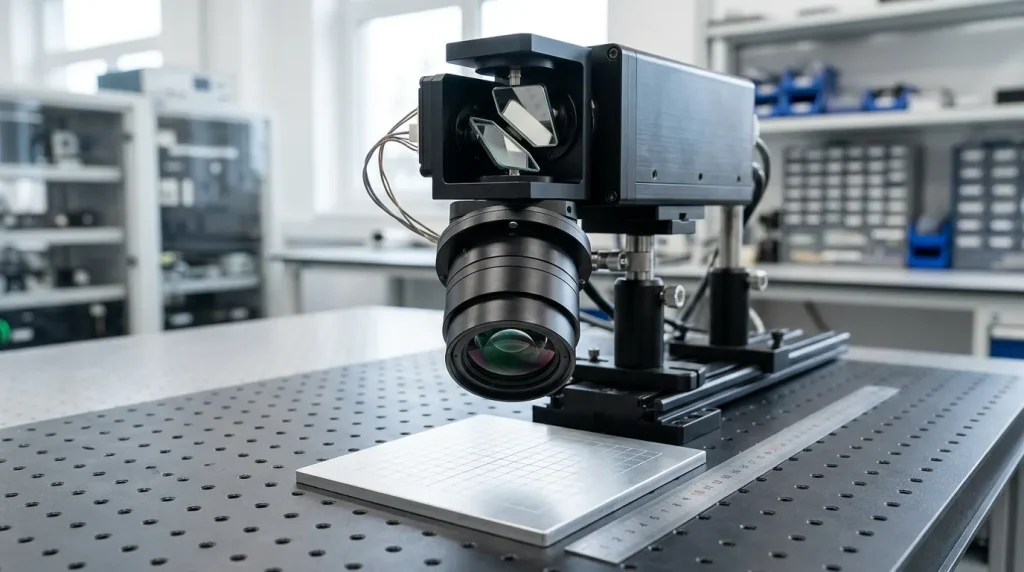
Engineers usually reach the question of how to calculate F-theta scan field size at one of two moments: when a marking field has to cover a part of known dimensions, or when a calculated field does not agree with the number printed on a lens datasheet. Both cases come down to the same short equation plus a set of conversions and physical limits that are easy to overlook. This article works through the calculation step by step, then explains why the geometric result is always an upper bound rather than a usable specification.
The Governing Equation
An F-theta lens is a flat-field scanning objective placed after a galvanometer scanner. It is deliberately designed with controlled barrel distortion so that the focused spot position on the work plane is proportional to the beam deflection angle rather than to its tangent.
Everything else in the calculation is bookkeeping: converting the angle into radians, confirming whether the quoted angle is optical or mechanical, deciding whether you need a half-field or a full field, and converting a round optical field into the rectangular working area a machine actually uses.
Step 1: Convert the Scan Angle to Radians
The equation y = fθ is only valid with θ in radians. Datasheets almost always quote degrees.
Substituting degrees directly into y = fθ inflates the result by a factor of about 57. It is the single most common arithmetic error in this calculation, and it is obvious once the result is compared against the lens housing diameter.
Step 2: Confirm Optical Angle Versus Mechanical Angle
A galvanometer mirror is a reflective element. Rotating it by a mechanical angle α deflects the beam by twice that angle:
Scan lens datasheets normally quote the optical scan angle. Galvo scanner datasheets normally quote the mechanical rotation angle. Mixing the two produces a field that is either half or double the correct value. A scanner rated at ±12.5° mechanical delivers ±25° optical to the lens, and it is the ±25° figure that belongs in the F-theta equation.
A second ambiguity is whether an angle is stated as a half-angle (±θ) or a full included angle (2θ). “Scan angle 40°” and “scan angle ±20°” describe the same lens. Where a datasheet is not explicit, the safest check is to divide the quoted scan length by the focal length and see which interpretation reproduces it.
Step 3: Calculate the Scan Length
The scan length, sometimes abbreviated SFD or called the scan field diameter, is the full sweep across the field centre in one axis:
Because the clear aperture of a scan lens is essentially rotationally symmetric, the maximum angle is available in every azimuth. The geometric field is therefore approximately a circle of that diameter, not a square. Mirror separation inside the scan head introduces a small asymmetry between the X and Y axes, so the field is close to circular but not perfectly so.
Step 4: Convert the Circular Field to a Usable Square Field
Most machines need a rectangular working area inscribed in that circle. The largest square that fits inside a circle has a side equal to the diameter divided by √2, and its diagonal equals the circle diameter:
Worked Examples: How to Calculate F-Theta Scan Field Size in Practice
Example A — Field from a known lens
A scan head is rated ±12.5° mechanical and is fitted with a 160 mm F-theta lens.
- Optical half-angle: 2 × 12.5° = 25° → 0.4363 rad
- Half field: 160 × 0.4363 = 69.8 mm
- Scan length: 2 × 69.8 = 139.6 mm
- Inscribed square: 139.6 ÷ 1.414 = 98.7 mm, so approximately 98 × 98 mm
The geometric limit is close to 100 × 100 mm, provided the lens itself accepts a ±25° optical input without vignetting. If the lens is only specified to ±20°, the scanner’s extra travel cannot be used and the field is limited by the optics, not the galvo.
Example B — Field across a focal length range
| Effective focal length | Half field y = fθ | Scan length (2y) | Inscribed square side |
|---|---|---|---|
| 63 mm | 22.0 mm | 44.0 mm | 31.1 mm |
| 100 mm | 34.9 mm | 69.8 mm | 49.4 mm |
| 163 mm | 56.9 mm | 113.8 mm | 80.5 mm |
| 254 mm | 88.7 mm | 177.3 mm | 125.4 mm |
| 420 mm | 146.6 mm | 293.2 mm | 207.3 mm |
The table shows the linearity that makes the calculation convenient: scan field scales directly with focal length at a fixed angle. It also shows the trade-off, because the focused spot diameter scales with focal length as well. A larger field obtained purely by increasing focal length gives up spot size and power density unless the input beam diameter is increased to compensate.
Reverse Calculation: Sizing the Focal Length for a Required Field
System designers usually run the calculation in the other direction. Rearranging:
Suppose a 200 × 200 mm square working area is required and the candidate lens family is specified to ±20° optical.
- Field diagonal: 200 × 1.414 = 282.8 mm
- Half diagonal: 141.4 mm
- Required focal length: 141.4 ÷ 0.3491 = 405 mm
The nearest longer standard focal length, such as 420 mm, provides margin. Note the difference made by the corner requirement: if only ±100 mm along each axis is needed and the corners of the square are not used, the required focal length falls to 100 ÷ 0.3491 = 286 mm. Deciding early whether the process genuinely uses the field corners can change the lens, the working distance and the achievable spot size substantially.
Why the Real Usable Field Is Smaller Than the Calculation
The geometric result assumes an unobstructed beam at every angle and acceptable optical quality out to the field edge. Four effects reduce it.
Vignetting and scanner mounting distance
As the beam is deflected, its footprint walks laterally across the lens entrance. For a pivot-to-lens-entrance distance L, the beam centre is displaced by L·tanθ, so the required entrance aperture is approximately:
This is why scan lens catalogues state the field for a specific scan head geometry or “aperture stop” distance. Moving the lens further from the mirrors, or fitting a scanner with wider mirror separation, clips the beam at large angles and shrinks the usable field even though the focal length has not changed.
Corner performance in a two-axis field
A point at the corner of a square field is reached by combining X and Y deflection, so the total off-axis angle at the corner is roughly √2 times the angle at the mid-edge. Aberrations, vignetting, spot ellipticity and transmission all degrade fastest there. The inscribed-square rule is not only geometry; it also keeps the extreme angle within what the design was corrected for.
Residual F-theta distortion
No lens follows y = fθ exactly. Distortion is normally specified as a percentage deviation from the ideal mapping:
In a two-axis system the residual is not a single number but a two-dimensional map, combining lens distortion with the pincushion-type error produced by the separation of the X and Y mirrors. Controllers compensate using a correction table generated for the installed lens, scan head and mounting distance. A low nominal lens distortion figure reduces the correction required but does not remove the need for system calibration.
Work-plane height and non-telecentric edge rays
In a standard, non-telecentric F-theta lens the chief ray at the field edge leaves at an angle to the surface normal. Raising or lowering the work plane by Δz therefore changes the field width by approximately 2·Δz·tan(θout) and shifts every point outward or inward. A field calibrated at one fixture height will not be dimensionally correct at another. Adding a protective window in the beam path also introduces a small focal shift that must be accounted for in the same way.
Why f·θ and Not f·tan θ
A conventional imaging lens maps field angle to image height as y = f·tanθ. If a scanning system used such a lens, the spot would accelerate toward the field edge under constant mirror angular velocity, changing the energy deposited per unit length. The magnitude is not negligible:
| Optical angle | θ in radians | tan θ | Deviation of f·tanθ from f·θ |
|---|---|---|---|
| 10° | 0.1745 | 0.1763 | +1.0% |
| 20° | 0.3491 | 0.3640 | +4.3% |
| 25° | 0.4363 | 0.4663 | +6.9% |
Some published descriptions of scanning lenses state that focus position depends on the tangent of the deflection angle. That describes the uncorrected behaviour the F-theta design exists to remove, and it should not be used to size a scan field.
Verifying Scan Field Size on a Real System
The calculation predicts the field; measurement confirms it. A practical verification sequence:
- Command the controller to mark a grid of known nominal pitch that extends to the intended field limits, using a stable target such as anodised aluminium or coated card.
- Measure the marked grid with a calibrated vision system, measuring microscope or CMM, and record the actual coordinates of each node.
- Compare actual against commanded positions to obtain the residual error map, then generate or update the controller correction file.
- Inspect spot geometry at the centre, mid-edge and corners. Ellipticity, power drop or visible clipping at the corners indicates vignetting rather than distortion, and defines the true usable field.
- Repeat at the production fixture height, with any protective window installed, since both change the result.
Common Calculation Mistakes
- Degrees left in the equation. θ must be in radians.
- Mechanical angle used as optical angle. Reflection doubles the deflection; the field comes out half its true size.
- Half-angle and full-angle confused. Check whether the datasheet means ±θ or 2θ.
- Circular field treated as a square field. The square side is the diameter divided by √2, not the diameter.
- Scanner geometry ignored. The published field assumes a specific mirror separation and lens mounting distance; changing either changes the vignetting limit.
- Working distance assumed equal to focal length. Effective focal length is measured from the principal plane; working distance is a mechanical dimension referenced to the housing.
- Full geometric field assumed to be fully usable. Edge and corner spot quality, not geometry, usually sets the process field.
Summary
Scan field size follows directly from y = fθ, but the useful engineering answer requires four consistent inputs: focal length, an optical scan angle in radians, the scanner geometry that determines vignetting, and a decision about whether the required field is circular, square by side, or square by diagonal. Calculate the geometric field first as an upper bound, then reduce it according to the lens acceptance angle and the measured edge performance. Where the calculated requirement sits between standard focal lengths or demands an unusual combination of field, working distance and spot size, the lens should be reviewed together with the scanner, beam expander and mechanical layout as one optical system rather than selected from a focal length alone.
Frequently Asked Questions
What is the formula for F-theta scan field size?
The spot position is y = f × θ, where f is the effective focal length in millimetres and θ is the optical scan angle from the optical axis in radians. The full one-axis scan length is 2 × f × θ, using the maximum optical half-angle. To obtain a square working area inscribed in that circular field, divide the scan length by √2. Degrees must be converted to radians first by multiplying by π/180, and the optical angle is twice the mechanical rotation of a galvanometer mirror.
Is a quoted scan field the square side or the field diagonal?
It depends on the supplier, which is why the figure should always be confirmed. A value expressed as “scan field diameter” or “scan length” is a one-axis sweep and equals the diagonal of the largest inscribed square. A value expressed as “110 × 110 mm” is normally the square side. The difference is a factor of √2, roughly 41%, which is large enough to invalidate a machine layout. Request the scan head geometry and mounting distance used for the published figure as well.
Does doubling the focal length double the scan field?
Geometrically yes, provided the same optical scan angle remains available without vignetting. In practice the longer lens must still accept the full angle, and a larger lens further from the scanner may clip the beam at extreme angles. Doubling focal length also approximately doubles the diffraction-limited focused spot diameter for the same input beam and wavelength, reducing power density. Field size and spot size cannot be optimised independently without changing the input beam diameter and scanner aperture.
Why is the catalogue scan field smaller than my calculation?
Published fields are usually derated below the geometric limit. Vignetting at large deflection angles, spot ellipticity and aberration growth at the field corners, transmission loss, residual distortion and the specific scan head geometry all reduce the usable area. Manufacturers commonly define the field at a stated maximum vignetting level and for one assumed mirror separation and mounting distance. Your calculation gives the theoretical upper bound; the catalogue value reflects performance that the design is prepared to specify.
Does changing the scan head change the field of the same lens?
Yes. The effective focal length is fixed, but the usable field is not. A different scan head changes the separation between the X and Y mirrors, the position of the effective pivot point and the distance from that pivot to the lens entrance. Those changes alter beam displacement at the lens aperture, and therefore where vignetting begins. They also change the two-dimensional distortion pattern, so the controller correction file must be regenerated after any scan head or mounting change.