
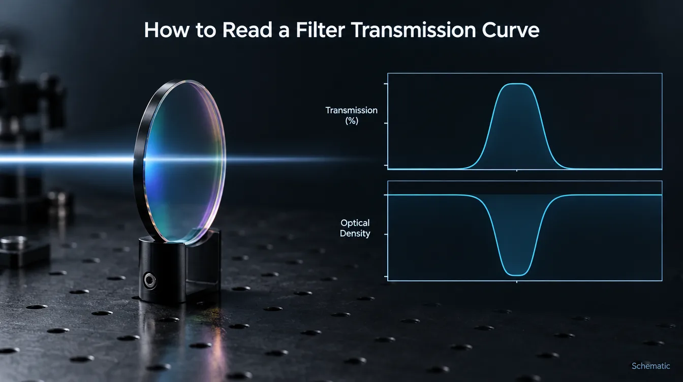
An optical filter transmission curve shows how much light the filter passes at each wavelength, but it proves performance only under the conditions it was measured. To read one correctly, check four things in order: what kind of curve it is, the test conditions (AOI, polarization, beam geometry, temperature), the vertical scale (linear %T or optical density), and only then the spectral features — CWL, FWHM, transmission and blocking — compared line by line with your specification.
Most disagreements between a filter buyer and a supplier do not come from a bad filter. They come from a curve read under one set of assumptions and a system that runs under another. The six checks below follow the order an optical engineer uses when a curve arrives with a sample, a datasheet or a test report.
Check 1: Identify what kind of curve you are looking at
Three different things are all called “the transmission curve”, and they do not carry the same weight.
| Curve type | What it represents | What it can verify |
|---|---|---|
| Design (theoretical) curve | The calculated response of the coating design, usually at 0° AOI with ideal layer thicknesses | That the design targets the right spectral shape. It verifies nothing about a manufactured part. |
| Typical curve | A representative plot published for a product type or family | The general behavior of that filter type. It is not acceptance data for a delivered lot. |
| Measured curve | A spectrophotometer scan of a specific part, sample or witness piece under stated conditions | The performance of that part, or of a lot if the sampling plan says so, under the stated test conditions |
Design curves usually look cleaner than reality: a flat passband, blocking that runs straight to the bottom of the plot, no ripple. A measured curve also contains substrate absorption, back-surface reflection, small layer errors and the limits of the instrument. If a curve carries no sample identification and no test conditions, treat it as illustrative, not as evidence.
One more distinction matters for coated parts: a witness piece coated in the same run is convenient to measure, but its position in the chamber, size and substrate can differ from the real part. Agree in advance whether the witness or the part itself is the acceptance sample.
Check 2: Read the test conditions before the shape
For an interference filter, the same part gives a different curve under different conditions. Before reading any wavelength off the plot, find these conditions on the curve or in the report:
- Angle of incidence (AOI). Most datasheet curves are measured at 0°. Tilting an interference filter moves its passband and edges toward shorter wavelengths.
- Polarization. At 0° it has no effect. At oblique incidence, s- and p-polarized light see different effective indices, so edges split and the passband shape changes. A curve labeled “unpolarized” or “average” is the mean of s and p, which is not what a polarized laser sees. See how polarization affects filter spectra at oblique incidence.
- Beam geometry. A spectrophotometer probes with a near-collimated or slowly converging beam. Behind a fast imaging lens, the filter sees a cone of angles, so the passband broadens, shifts toward shorter wavelengths and loses peak transmission. See the cone half-angle effect on interference filters.
- Temperature. Interference filters drift slowly with temperature. For narrowband filters in instruments that run hot or cold, a room-temperature curve may not describe the operating condition.
- Wavelength range, step and instrument spectral bandwidth. These decide what the curve can and cannot show (Checks 4 and 5).
For collimated light, the first-order estimate of the angle shift is:
Here λ0 is the wavelength at normal incidence, θ is the AOI in air, and neff is the effective index of the coating design. neff depends on the layer materials and design, and differs for s and p polarization; ask the supplier for it or, better, for a curve at the real angle.
Illustrative example (calculated, not measured data): shift toward shorter wavelength for a feature at 850 nm at normal incidence.
| AOI | Shift, neff = 1.8 | Shift, neff = 2.0 |
|---|---|---|
| 5° | ≈ 1.0 nm | ≈ 0.8 nm |
| 10° | ≈ 4.0 nm | ≈ 3.2 nm |
| 15° | ≈ 8.8 nm | ≈ 7.1 nm |
| 20° | ≈ 15.5 nm | ≈ 12.5 nm |
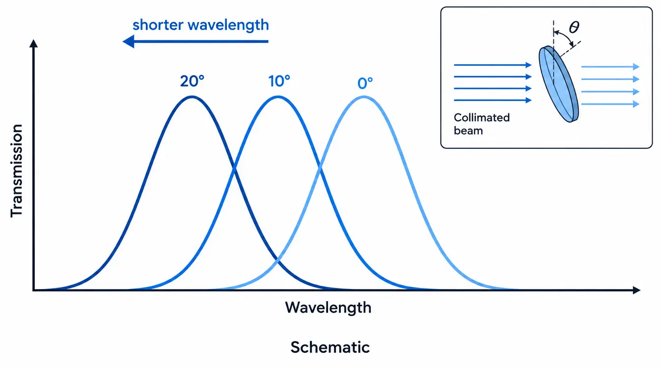
Read the shift against the bandwidth. A 3–4 nm move at 10° hardly matters for a 50 nm wide bandpass filter, but it can push a 10 nm FWHM narrowband filter partly off a laser line, especially once laser wavelength tolerance and temperature drift are added.
Check 3: Check the vertical axis — linear %T or optical density
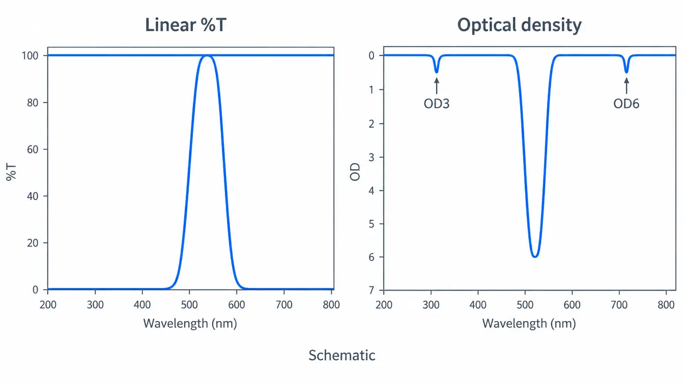
A linear transmission axis (0–100%) is where you read the passband. It is almost useless for blocking: 0.1% and 0.0001% both sit on the baseline and look identical.
Blocking is read in optical density:
where T is transmittance as a fraction, not a percentage.
| OD | Transmittance (fraction) | Transmittance (%) |
|---|---|---|
| 1 | 0.1 | 10% |
| 2 | 0.01 | 1% |
| 3 | 0.001 | 0.1% |
| 4 | 0.0001 | 0.01% |
| 5 | 0.00001 | 0.001% |
| 6 | 0.000001 | 0.0001% |
When you read a blocking region:
- Judge an OD specification only on an OD or log-scale plot, or a data table. A spec such as “OD4 from 400 to 800 nm” cannot be confirmed on a linear plot.
- Find where the axis ends. If the plot stops at OD5, a curve touching the bottom only shows that blocking reaches about the limit of the plot, not its real value.
- Suspect a flat, noisy floor. A constant OD level across a wide range often marks the instrument’s noise floor rather than the coating. Conventional spectrophotometers also round off very steep edges, and imperfect monochromator gratings can let passband light into the measurement near a steep edge, so the blocking right next to the passband reads shallower than it is (IDEX Health & Science).
If a project needs deep blocking, agree on the measurement method and its dynamic range before production, not after the first lot. For the trade-offs behind high OD values, see OD4 vs OD6.
Check 4: Read the passband parameters the way your specification defines them
Many curve disputes are definitional. Before comparing a number with the spec, make sure both sides mean the same thing.
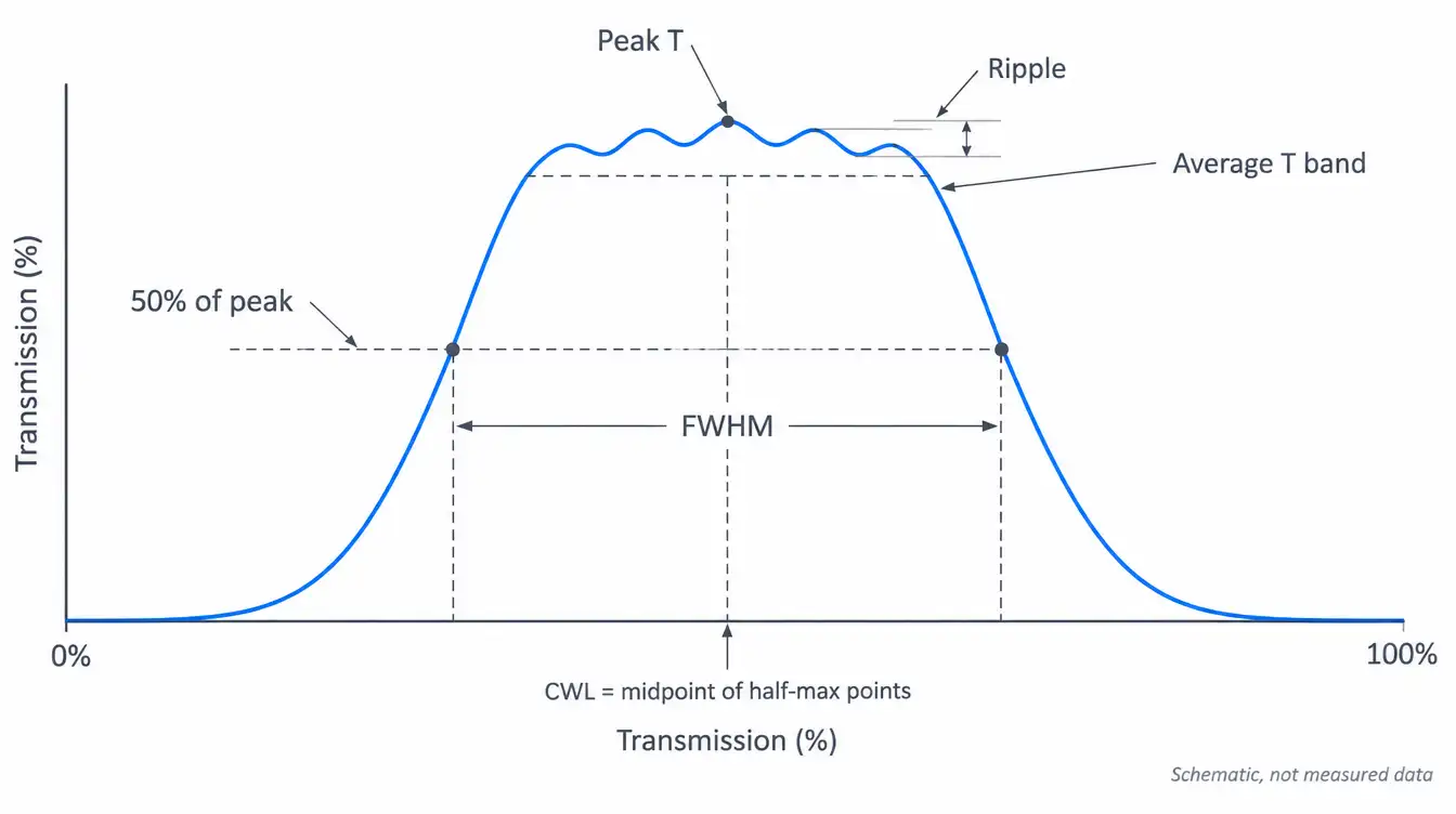
- Peak transmission (Tpeak) is the single highest point in the passband.
- Average transmission (Tavg) is the mean over a stated wavelength range. Ripple in the passband makes Tavg lower than Tpeak, so a spec of “T > 90%” must say which one it means and over what range.
- FWHM is the passband width at half of the peak transmission. If Tpeak is 90%, read the width at 45%, not at 50%.
- CWL is normally the midpoint between the two half-maximum wavelengths, not the wavelength where transmission is highest. On an asymmetric or rippled passband, the two can differ.
- Cut-on and cut-off wavelengths of longpass and shortpass filters are usually taken at a 50% level. Check whether that means 50% absolute or 50% of the passband transmission.
- Edge steepness is defined between two levels, for example 10% to 90%, or 50% to a stated OD. Compare two filters only when both use the same levels. See edge steepness in an optical filter.
Two measurement effects also change these numbers:
- Instrument spectral bandwidth. The recorded curve is the real filter response smeared by the instrument’s own bandwidth. When that bandwidth is not small compared with the FWHM, the peak reads lower, the band reads wider and the edges look softer. This matters most for narrowband and steep-edge filters, so check the slit or bandwidth setting on the report. As a reference point, ASTM E958, written for absorbance measurements, asks for an instrument bandwidth below about one-eighth of the band’s half-width; a similar margin is a sensible target when measuring narrow passbands.
- Back-surface reflection. A measured curve covers the whole part. An uncoated glass surface with n ≈ 1.5 reflects about 4% at normal incidence, so a filter with an uncoated back side cannot show the same peak as a design curve calculated for the coating alone.
When a CWL or FWHM sits near the edge of its tolerance, the measurement conditions above decide whether the part passes. For how tolerances are written, see optical filter spectral tolerance explained.
Check 5: Check blocking across the range your system can actually detect
A curve verifies only the wavelengths it shows. The range that matters is where your light source emits and your detector responds, including ambient light that reaches the sensor.
A silicon sensor responds out to roughly 1,100 nm. A bandpass curve plotted only to 1,000 nm says nothing about leakage at 1,064 nm, even if the plotted region looks perfect. InGaAs detectors extend the range of concern further into the SWIR.
This matters because an interference bandpass coating has secondary transmission regions away from its main band. Blocking over a wide range is usually extended with additional blocking coatings or absorbing glass, and the curve should show that extended range on an OD scale. For how to write that range into a specification, see how to specify OD blocking range for a bandpass filter.
Check 6: Compare the curve with the specification, line by line
Once the curve type, conditions and definitions are clear, the comparison itself is straightforward.
| Spec item | Read on the curve | Common reading error |
|---|---|---|
| CWL ± tolerance | Midpoint of the half-maximum points, at the specified AOI | Reading the peak wavelength; using a 0° curve for a tilted mount |
| FWHM ± tolerance | Width at half of peak transmission | Reading at 50% absolute on a lower-transmission filter |
| Tpeak or Tavg | Highest point, or mean over the stated band | Treating a peak value as an average |
| Blocking OD over a range | OD plot across the full stated range | Judging from a linear plot; reading the instrument floor as filter OD |
| Cut-on / cut-off | 50% point by the stated definition | Mixing absolute and relative 50% levels |
| AOI, polarization, cone angle | Stated on the curve or in the report | Missing conditions treated as “0° is fine” |
Anything the curve does not show — blocking outside the plotted range, a different AOI, the operating temperature — is not verified by that curve. It needs another measurement, an agreed design calculation, or a stated exclusion in the specification.
Common misreadings that cause problems in the field
- Comparing two suppliers’ curves as if they were measured the same way. Different instrument bandwidth, AOI or polarization can make the same filter look better or worse.
- Using a typical or design curve for incoming inspection. It shows what the product type should do, not what the delivered lot did.
- Checking only the passband. A clean visible-range curve can hide a near-infrared leak that a silicon sensor sees clearly.
- Ignoring the mount. A filter tilted to send back-reflections out of the path, or placed in a converging beam, runs at conditions the 0° curve never measured.
What a verification-ready transmission curve should state
A curve that can be used to accept or reject parts usually states:
- Sample identification: part, lot, or witness piece
- AOI, polarization state and beam geometry (collimated or cone half-angle)
- Measurement temperature, if the application is temperature-sensitive
- Instrument type, spectral bandwidth and wavelength step
- Wavelength range covered, and the scale used (linear %T, log or OD) with its floor
- The definitions used for CWL, FWHM, Tavg and edge positions
- The acceptance criteria the curve is checked against
Defining the test curve before the order
The simplest way to avoid curve disputes is to agree on the test conditions and definitions before production. GIAI reviews custom optical projects against the drawing, sample, optical requirements, substrate, geometry, coating conditions and inspection criteria before defining the manufacturing route. For filters, spectral verification is set according to the project specification — transmission, blocking, CWL, FWHM, AOI and other agreed characteristics — and the test conditions should match the final application or the agreed specification. The Quality Assurance page outlines how that verification fits into the inspection flow.
For a custom filter, send the drawing or specification together with the wavelength range, CWL and FWHM or edge positions, required blocking OD and its wavelength range, AOI and cone angle, polarization, operating temperature, substrate, dimensions, the required test conditions and report format, and the expected quantity. Contact GIAI for a technical review.
FAQ
What is the difference between a transmission curve and an OD curve?
Both show the same measurement on different vertical scales. A transmission curve plots T in percent on a linear axis, which makes the passband easy to read. An OD curve plots −log10(T), which stretches the low-transmission region so blocking levels such as OD4 (0.01%) and OD6 (0.0001%) can be told apart. Use the linear plot for CWL, FWHM and passband transmission, and the OD plot for blocking.
Why does my measured CWL differ from the datasheet?
The usual causes are a different AOI, a converging beam instead of collimated light, polarization at oblique incidence, a different temperature, or a different CWL definition (peak wavelength instead of the midpoint of the half-maximum points). Instrument calibration and spectral bandwidth also contribute. Compare the two curves only after matching these conditions.
Can I verify OD6 blocking from a standard spectrophotometer scan?
Only if the instrument’s dynamic range and noise floor go well beyond the level being claimed. On many conventional setups, a curve that flattens at a constant OD shows the instrument limit, not the filter. For deep blocking, agree on the test method and how results are reported before the order.
Does a design curve guarantee the manufactured filter will match it?
No. A design curve is a calculation for ideal layers and a stated AOI. Real parts differ through layer thickness errors, substrate absorption, back-surface reflection and the measurement setup. Acceptance should rest on measured data under agreed conditions.
Is transmittance the same in both directions through a filter?
For a stable, linear filter, transmittance is generally the same in either direction, but reflectance from the two sides can differ, and so can heating in absorbing glass and stray reflections in the system. Orientation is therefore still worth specifying; see optical filter orientation and the coated side.